
Information on the HMB method of Valve Lift Design. (Back)
With
Reference to Fig.1 ...
Although the design procedure for the HMB and GPB methods for the valve
lift profile are different the design process in all three cases is identical.
Hence, in this explanation for the HMB method, the same explanations do
not have to be repeated for the others. Fig.1 below shows the front
page of the HMB method for both input and output data control and the
on-screen design procedures one wishes to observe.
NOTE P1.1: The user can select any one of three types of ramp;
cosine being an old-fashioned trigonometric procedure, constant
velocity being the most common, and acceleration
often effective in racing designs. The ramps at valve opening and closing
can be designed to be different at each end.
NOTE P1.2: The design is conducted at a camshaft speed as some
design criteria, such as ramp velocity or valvetrain dynamics computations,
require cycle time as a data input for optimisation purposes.
NOTE P1.3: The optimisation of ramp velocity, usually conducted
at the highest operational camshaft speed, is normally expressed in terms
of a velocity in units of m/s, ft/sec, or even mph! The optimum maximum
ramp velocity is typically in the range of 1.0 to 1.5 m/s but this only
becomes a logical design procedure if the valve lash selected falls within
its operational ambit. The selection of valve lash (clearance) will be
discussed below in relation to Fig.4.
NOTE P1.4: The user may insert a valve lift and the computation
delivers the open-close duration at that valve lift and the aggression
of that valve lift profile in terms of the lift-duration envelope ratio,
Kld. Aggression is directly related to cylinder filling and emptying for
that valve.
NOTE P1.5: The user may select up three levels of smoothing of
the valve lift profile; this will be discussed in detail in Fig.3.
NOTE P1.6: The user may import a previous valve lift profile design
and have it directly compared with the current design as the design proceeds
this will be discussed in detail in Figs.6 and 7.
NOTE P1.7: The 'data info' button contains very extensive 'help
files'.
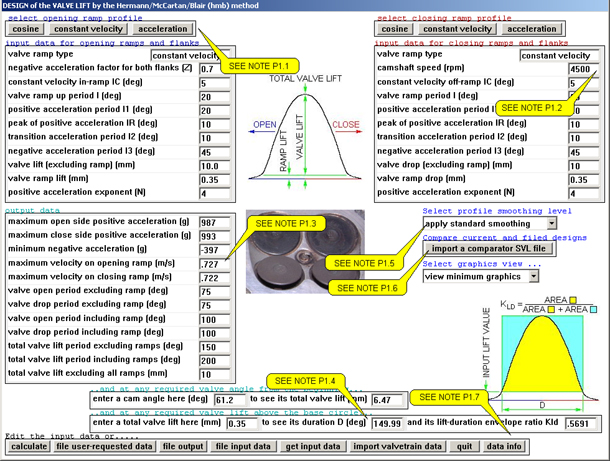 Figure
1. Front Page of the HMB Method
Figure
1. Front Page of the HMB Method
With
Reference to Fig.2 ...
This graphic of the valve lift design appears upon a ' calculation'. It
is the result of using the input data in Fig.1. The ramp selected
is a 'constant velocity' ramp and the flat shape at the ramp mid-point
reflects the name; by definition the acceleration here is zero as is the
force moving it. The spaces between the vertical green lines are the ramp
periods (I or I+IC), the positive acceleration period (I1), the transition
acceleration period (I2) and the negative acceleration period (I3); all
X and Y data are graphed to scale and any Y data is scaled to its local
maximum.
NOTE P2.1: The vertical black line is at an angle where the valve
lift is precisely 0.35 mm (as selected in Fig.1 at NOTE P1.4).
The black line at the right also crosses the lift at precisely 0.35 and
the interval between them is 149.99 deg and the Kld aggression level between
them is 0.5691 (see Fig.1).
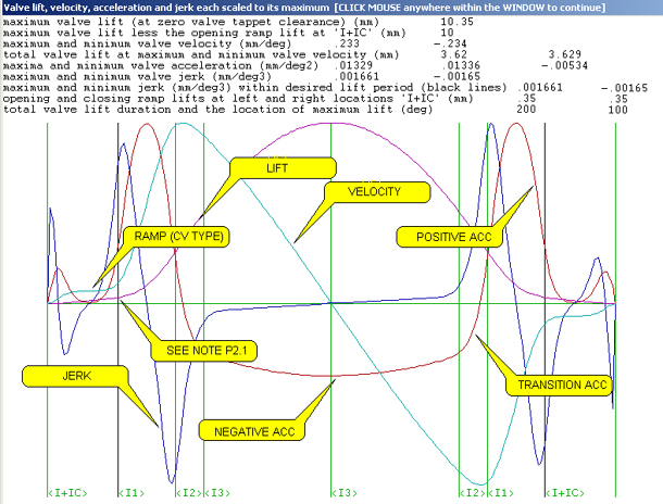
Figure
2. Graphic of Valve Lift Design
With
Reference to Fig.3 ...
Fig.3 below illustrates the quality of the smoothing that exists within
the 4stHEAD software . Three levels of smoothing may be selected (see
NOTE P1.5). Screen snapshots are given here of using these three
smoothing levels (minimal, standard or heavier) and their effect on the
maximum acceleration and jerk levels on the valve lift profile. The effect
on the shape of the rising positive acceleration curve is quite obvious
and the numerical shift of the maximum jerk value is some 50%. Jerk is
the rate of change of acceleration, or force, and so jerk is a measure
of the high frequency chatter of the valve, valve follower and tappet-cam
contact forces. By definition, jerk is also directly related to valvetrain
noise and so, while heavier smoothing will be in design use for standard
automotive valvetrain design, standard or minimal smoothing will be used
for racing engine design. It will be observed that the several levels
of smoothing barely effect the maximum values of acceleration.
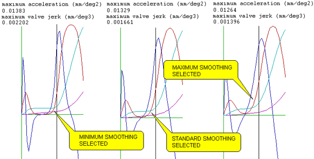
Figure
3. The Effect of Smoothing on the Acceleration Curve
With
Reference to Fig.4 ...
Fig.4 below shows screen snapshots of two differing values of selected
valve lift, namely 0.35 mm and 0.2 mm. The black line crosses the lift
graph at precisely those lift values. The 0.35 lift value is the value
of the designed ramp lift (see Fig.1) and it is rather obvious
that the designer would not use this value as the valve lash (tappet clearance)
as the black line indexes the jerk curve near its maximum and the acceleration
(force) graph at some 25% of its maximum. However, a valve lash setting
of 0.2 mm, or some 0.15 mm or 0.006 inch less, lies on the flat of the
CV ramp and at zero jerk and acceleration.
NOTE P4.1: The designer can change the selected valve lift and,
by observing the conjunction of the 'black lift line' and the flat part
of the CV ramp, may precisely establish the valve lash and the numerical
tolerance for its setting.
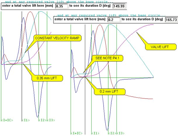
Figure
4. Snapshots
of Two Differing Values of Selected Valve Lift Using CV Ramp
With
Reference to Fig.5 ...
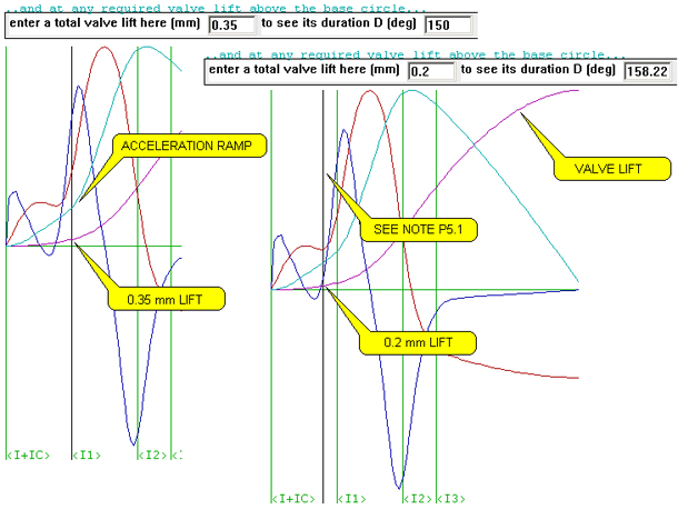
Fig.5 below illustrates the equivalent discussion to that for Fig.4
with its constant velocity ramp design. Here, in Fig.5, the ramp
design has been selected as an acceleration ramp (see NOTE P1.1).
The definition of an acceleration ramp is one of linearly increasing velocity
and that definition can be seen to be executed numerically in Fig.5.
The optimum valve lash setting is still 0.2 mm so as to give virtually
zero jerk and 'low' acceleration (force) at cam to tappet contact but
the tolerance window of camshaft angle contact to satisfy this criterion
is not so wide as for a CV ramp.
NOTE P5.1: Hence, acceleration ramp design is normally reserved
for racing engines whereas CV ramps can be applied universally. However,
short period, low lift, acceleration ramps see significant design application
for valve lift profiles with hydraulic tappets.
Figure
5. Snapshots
of Two Differing Values of Selected Valve Lift Using Acceleration Ramp
With
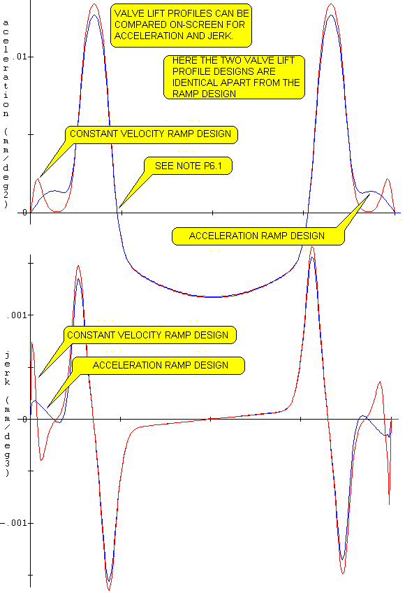
Reference to Fig.6 ...
In NOTE P1.6 it is pointed out that it is possible to import a
valve lift profile and compare it continuously with a current design as
the design process for it proceeds. In this case (Fig.6 below)
the imported design is the CV ramp design from the input data used thus
far (as in Fig.1) and the immediate design modification is to change
both ramps to acceleration ramps with all other data kept identical. The
fundamental differences in the two acceleration diagrams is very obvious
as is that for the jerk diagrams. On the jerk diagram, the valve lash
location of 'zero jerk' is clearly visible. These on-screen pictures of
acceleration and jerk are invaluable during a real design process where
one is attempting to improve on an existing design.
NOTE P6.1: It is interesting to note in this particular case that
the valve lift profile with the constant velocity ramp yields higher acceleration
and jerk values than that with the acceleration ramp; this is not a universal
law!
Figure
6. Comparison
of Acceleration and Jerk Diagrams for a CV Ramp and Acc Ramp
With
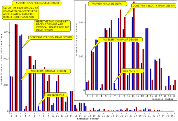
Reference to Fig.7 ...
Fig.7 below continues the theme of 'comparison of valve lift profiles
during design' where the information conveyed to the designer in Fig.6
is further enhanced by conversion via a Fourier analysis into harmonics
up to the 36th. The amplitude of each harmonic is drawn on the two bar
charts.
NOTE P7.1: It is observed that the 4th, 7th and 10th harmonics
have low amplitudes on the Fourier analysis of the acceleration diagram
and similarly on the jerk bar chart. At the selected camshaft speed of
4500 rpm (see NOTE P1.2) or 75 Hz (rps), then the 4th harmonic
is 300 Hz, the 7th is 525 Hz and the 10th is 750 Hz. Valve springs typically
have natural frequencies in the 400 to 800 Hz range and so this particular
valve lift profile would be very happy to attempt to vibrate valve springs
whose natural frequencies were 525 and/or 750 Hz when the engine was turning
at 9000 rpm; with low harmonic acceleration (force) and jerk levels they
would be hard to excite into any damaging resonance!
Figure
7. Comparison
of Fourier Analyses of Acceleration and Jerk Diagrams for a CV Ramp and
Acc Ramp
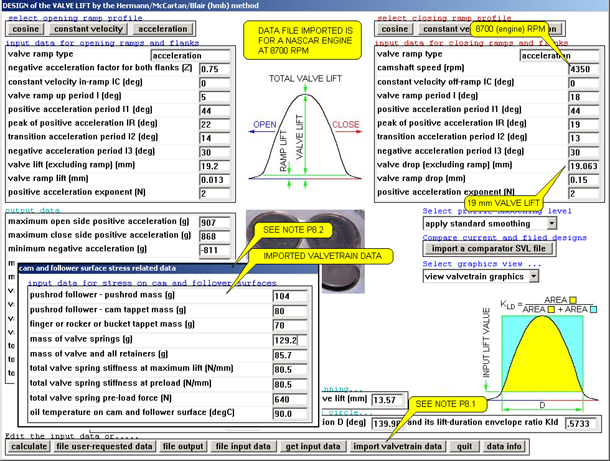
With
Reference to Fig.8 ...
On the front input data page, as in Fig.1, it can be seen that
a control button exists to 'import valvetrain data'.
NOTE P8.1: Superimposed on Fig.8 below is the 'valvetrain
data' that one has imported. It is created in fine detail in PROGRAM NO.10
(the specialist analysis for valvetrain dynamics) and exported to PROGRAM
NO.9 (cam design and manufacture) because without a static analysis of
the dynamic events on cam to follower contact it is not possible to compute
the oil film thickness nor the Hertzian stresses. From there that very
same force and component mass data can be imported into PROGRAMS NO.1-3
where a mini-dynamic analysis on the entire valvetrain can be quickly
conducted to ascertain if the designed valve lift profile has any possibility
of controlling the selected valvetrain at the engine speed required.
NOTE P8.2: This input/imported data table is actually a screen
dump from PROGRAM NO.9 and is not visible when importing the valvetrain
data in PROGRAMS NO.1-3 as much more data than this is being invisibly
(to the designer) transferred at the same juncture, if applicable., viz
rocker geometry, pushrod geometry, or finger geometry, etc. Please note
the input data is for a NASCAR pushrod racing engine with a valve lift
of some 19 mm running at 8700 rpm.
Figure
8. Front
Page of the HMB Method with Imported Valvetrain Data
With
Reference to Fig.9 ...
When the design computation is for the current valve lift profile is indexed
so too is the 'mini-dynamic valvetrain dynamics' calculation. It is quite
complex and takes perhaps 10 seconds to execute on a fast PC; this is
in contrast to the complete and extremely detailed valvetrain dynamics
computation in PROGRAM NO.10 for the very same valvetrain that might take
5 minutes on the same fast PC. What emerges is the screen graphic shown
here for acceleration (g) with static (black) and dynamic accelerations
(red) running up to 1000 g for the valve.
NOTE P9.1: In several software packages which are commercially
available they report that they design the valve spring deceleration (spring
preload plus spring stiffness times its compression which force is then
converted to a system deceleration) and plot this as the dark blue (static
deceleration) line on Fig.9. Their design decision is based on
this deceleration being less than the static deceleration at maximum valve
lift, as in the case being shown here, in which case they confidently
assert that that the valve cannot 'loft'. However, in this case when we
plot the dynamic deceleration from the computation (the pale blue line)
it can be seen that the valve springs have lost control of the valve just
before maximum valve lift and so the valve will loft.
NOTE P9.2: Perhaps even worse, after maximum valve lift there is
an excess of force (pale blue lower than red) returning the valve to its
seat; it may well bounce. In short, for our software competitors to rely
on static deceleration for a design decision on dynamic behaviour does
not constitute a logical design procedure. Equally, and in the same vein,
on the web pages of these same software competitors, or in their technical
publications, you do not find valve lift profile designs presented with
the same degree of numerical clarity or graphical visibility for their
lift, velocity, acceleration or jerk data, nor do you find examples of
the quality of the smoothing of their valve lift profiles nor critical
debates on optimum ramp design, Fourier analysis, etc., etc.
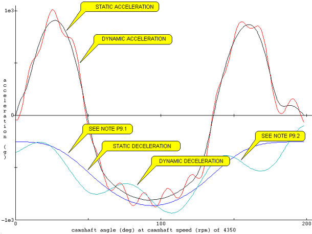
Figure
9. Graphical
Results of a 'Mini-Dynamic Valvetrain Dynamics' Calculation

©Prof Blair & Associates